Dies ist eine Frage der Geschwindigkeit. Ich versuche, eine Diffusionsgleichung zu lösen, die in dem drei Verhalten Zustände hat:4. Bestellung Runga Kutta Methode - Diffusionsgleichung - Bildanalyse
- Lambda == 0 Gleichgewicht
- Lambda> 0 max Diffusion
- Lambda < 0 min Diffusions
Engpass ist die else-Anweisung in der Diffusionsoperatorfunktion
Der Gleichgewichtszustand hat einen einfachen T-Operator oder und Diffusionsoperator. Für die anderen beiden Staaten wird es ziemlich kompliziert. Und bisher hatte ich nicht die Geduld, die Code-Laufzeiten zu überstehen. Soweit ich weiß, sind die Gleichungen korrekt, und die Ausgabe des Gleichgewichtszustandes erscheint korrekt, vielleicht hat jemand einige Tipps, um die Geschwindigkeit für die Nicht-Gleichgewichtszustände zu erhöhen?
(Euler-Lösung (FTCS) anstelle von Runge-Kutta wäre schneller ich mir vorstellen. Haben Sie nicht versucht diese noch.)
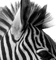
Sie können eine beliebige Schwarz-Weiß-Bild importieren Sie den Code heraus zu versuchen.
import numpy as np
import sympy as sp
import scipy.ndimage.filters as flt
from PIL import Image

# import image
im = Image.open("/home/will/Downloads/zebra.png")
arr = np.array(im)
arr=arr/253.

def T(lamda,x):
    """
    T Operator
    lambda is a "steering" constant between 3 behavior states
    -----------------------------
    0  -> linearity
    +inf -> max
    -inf -> min
    -----------------------------
    """
    if lamda == 0: # linearity
     return x
    elif lamda > 0: # Half-wave rectification
     return np.max(x,0)
    elif lamda < 0: # Inverse half-wave rectification
     return np.min(x,0)


def Diffusion_operator(lamda,f,t):
    """
    2D Spatially Discrete Non-Linear Diffusion
    ------------------------------------------
    Special case where lambda == 0, operator becomes Laplacian


    Parameters
    ----------
    D : int      diffusion coefficient
    h : int      step size
    t0 : int      stimulus injection point
    stimulus : array-like  luminance distribution

    Returns
    ----------
    f : array-like    output of diffusion equation
    -----------------------------
    0  -> linearity (T[0])
    +inf -> positive K(lamda)
    -inf -> negative K(lamda)
    -----------------------------
    """
    if lamda == 0: # linearity
     return flt.laplace(f)
    else:   # non-linearity
     f_new = np.zeros(f.shape)
     for x in np.arange(0,f.shape[0]-1):
      for y in np.arange(0,f.shape[1]-1):
       f_new[x,y]=T(lamda,f[x+1,y]-f[x,y]) + T(lamda,f[x-1,y]-f[x,y]) + T(lamda,f[x,y+1]-f[x,y])
       + T(lamda,f[x,y-1]-f[x,y])
     return f_new


def Dirac_delta_test(tester):
    # Limit injection to unitary multiplication, not infinite
    if np.sum(sp.DiracDelta(tester)) == 0:
     return 0
    else:
     return 1

def Runge_Kutta(stimulus,lamda,t0,h,N,D,t_N):
    """
    4th order Runge-Kutta solution to:
    linear and spatially discrete diffusion equation (ignoring leakage currents)

    Adiabatic boundary conditions prevent flux exchange over domain boundaries
    Parameters
    ---------------
    stimulus : array_like input stimuli [t,x,y]
    lamda : int    0 +/- inf
    t0 : int    point of stimulus "injection"
    h : int     step size
    N : int     array size (stimulus.shape[1])
    D : int     diffusion coefficient [constant]

    Returns
    ----------------
    f : array_like   computed diffused array

    """
    f = np.zeros((t_N+1,N,N)) #[time, equal shape space dimension]
    t = np.zeros(t_N+1)

    if lamda ==0:
     """ Linearity """
     for n in np.arange(0,t_N):
      k1 = D*flt.laplace(f[t[n],:,:]) +  stimulus*Dirac_delta_test(t[n]-t0)
      k1 = k1.astype(np.float64)
      k2 = D*flt.laplace(f[t[n],:,:]+(0.5*h*k1)) +  stimulus*Dirac_delta_test((t[n]+(0.5*h))- t0)
      k2 = k2.astype(np.float64)
      k3 = D*flt.laplace(f[t[n],:,:]+(0.5*h*k2)) + stimulus*Dirac_delta_test((t[n]+(0.5*h))-t0)
      k3 = k3.astype(np.float64)
      k4 = D*flt.laplace(f[t[n],:,:]+(h*k3)) + stimulus*Dirac_delta_test((t[n]+h)-t0)
      k4 = k4.astype(np.float64)
      f[n+1,:,:] = f[n,:,:] + (h/6.) * (k1 + 2.*k2 + 2.*k3 + k4)
      t[n+1] = t[n] + h
     return f

    else:
     """ Non-Linearity THIS IS SLOW """
     for n in np.arange(0,t_N):
      k1 = D*Diffusion_operator(lamda,f[t[n],:,:],t[n]) + stimulus*Dirac_delta_test(t[n]-t0)
      k1 = k1.astype(np.float64)
      k2 = D*Diffusion_operator(lamda,(f[t[n],:,:]+(0.5*h*k1)),t[n]) + stimulus*Dirac_delta_test((t[n]+(0.5*h))- t0)
      k2 = k2.astype(np.float64)
      k3 = D*Diffusion_operator(lamda,(f[t[n],:,:]+(0.5*h*k2)),t[n]) + stimulus*Dirac_delta_test((t[n]+(0.5*h))-t0)
      k3 = k3.astype(np.float64)
      k4 = D*Diffusion_operator(lamda,(f[t[n],:,:]+(h*k3)),t[n]) + stimulus*Dirac_delta_test((t[n]+h)-t0)
      k4 = k4.astype(np.float64)
      f[n+1,:,:] = f[n,:,:] + (h/6.) * (k1 + 2.*k2 + 2.*k3 + k4)
      t[n+1] = t[n] + h

     return f

# Code to run
N=arr.shape[1] # Image size
stimulus=arr[0:N,0:N,1]
D = 0.3 # Diffusion coefficient [0>D>1]
h = 1  # Runge-Kutta step size [h > 0]
t0 = 0 # Injection time
t_N = 100 # End time

f_out_equil = Runge_Kutta(stimulus,0,t0,h,N,D,t_N)
f_out_min = Runge_Kutta(stimulus,-1,t0,h,N,D,t_N)
f_out_max = Runge_Kutta(stimulus,1,t0,h,N,D,t_N)
Kurz gesagt, ist f_out_equil relativ schnell zu berechnen, während Min- und Max-Fälle sind teuer und langsam.
Hier ist ein Link zu einem Bild, das ich verwendet habe: meine Codierung geschätzt, Vielen Dank auf der Verbesserung der http://4.bp.blogspot.com/_KbtOtXslVZE/SweZiZWllzI/AAAAAAAAAIg/i9wc-yfdW78/s200/Zebra_Black_and_White_by_Jenvanw.jpg
Tipps,
Hier ist ein schnelles Plotten Skript für die Ausgabe
import matplotlib.pyplot as plt
fig1, (ax1,ax2,ax3,ax4,ax5) = plt.subplots(ncols=5, figsize=(15,5))
ax1.imshow(f_out_equil[1,:,:],cmap='gray')
ax2.imshow(f_out_equil[t_N/10,:,:],cmap='gray')
ax3.imshow(f_out_equil[t_N/2,:,:],cmap='gray')
ax4.imshow(f_out_equil[t_N/1.5,:,:],cmap='gray')
ax5.imshow(f_out_equil[t_N,:,:],cmap='gray')
Sind Sie sicher, dass Ihr Code korrekt ausgeführt wird? Es gibt Klammern in den letzten paar Zeilen – Alessandro
sollte jetzt gut sein – WBM
Ich bekomme einen Formfehler mit dem ersten Zebra s/w Bild, das ich bei Google gefunden habe, vielleicht können Sie eine Dateiverbindung bereitstellen, die für Ihr Beispiel funktioniert. – Alessandro